Analysis of Menard pressuremeter results in a spectral diagram

SUMMARY -

The rules for using the values of the_EM modulus and the limit pressure P*LM in the pressuremeter method require the user to take the_EM/P*LM ratio into consideration when classifying soils, and in particular to set the value of the rheological coefficient α, a decision whose consequence is important for the predictions of settlement and other deformations. The proposed graphical representation has been an aid for this choice for more than a decade.

1. Fundamental character of the ratio between_EM and_PLM and the rheological coefficient α

Louis Ménard chose to define the deformation modulus, which today bears his name, from the pressuremeter test instead of the shear modulus, which results directly from the equation for the expansion of a cylindrical cavity in an elastic medium (Lamé, 1852):

where

• G is the shear modulus for the range of induced stresses,
• R is the radius of the straight section of the hole, 
• ∆R denotes the increase in this radius as a function of a pressure increase ∆p at the cavity wall,
  by choosing the conventional fixed value ν =1/3 for soils for the Poisson's ratio that links orthogonal deformations.

He also emphasised the importance of the link between the strain rate and the fracture resistance of a soil, which could be overlooked by reducing the pressuremeter test to the measurement of its two parameters_EM and_PLM. He defined the type of soil behaviour in terms of the dimensionless_EM/PLM ratio, related to the rheological coefficient α, such that α =_EM/Ey, in a table to help decide on the value of α as a function of_EM/PLM and the nature of the soil (Ménard and Rousseau, 1962).

To date, no more precise method of determining α has been proposed. This could have been expected, for example, from systematic comparisons between pressure modulus and oedometer measurements, a subject on which publications of experimental results remain sporadic and bearing in mind that the oedometer modulus is variable according to the pressure range for which it is defined.

The range of values that the_EM/PLM ratio can take for common pressuremeter tests is relatively limited: the extreme values in Menard's original table range from 6 (normally consolidated sands and gravels) to 16 (overconsolidated clay), and the idea that the average is 10 is sufficiently accredited that tests that deviate too far from this average are sometimes considered questionable. And indeed, reshaping a ring of soil around the borehole will tend to cause the_EM/PLM ratio to fall sharply, while improperly sinking the probe into clay soil will raise the pore pressure and artificially increase the_EM/PLM ratio which can reach high or very high values.

In other words, apart from those cases that can be detected during the test and especially the drilling, the correlation between_EM and_PLM is often strong.

2. Interest of a graphic representation

2.1 Graph of_EM versus_PLM  

The graphical representation of_EM as a function of_PLM on the x-axis of a large number of tests in weathered soils and rocks (Figure 1a) is of little use in differentiating between tests, but shows this concentration of representative points.

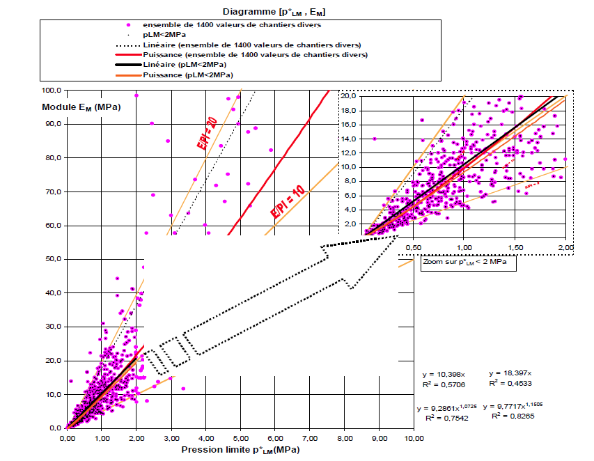
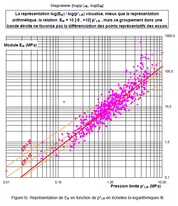
A representation [log(_PLM), log(_EM)] differentiates the representative points a little better (Figure 1b), which however remain grouped in the narrow band between_EM /P*LM = 5 and_EM /P*LM = 20, which become in this bi-logarithmic frame of reference parallel straight lines.

2.2 Graph of_EM / P*LM versus P*LM 

In order to visually distinguish the representative points of pressuremeter tests in a more "spread out" diagram, we propose to systematically plot the representative points of pressuremeter tests of the same soil, borehole or site in a bi-logarithmic diagram [log(_EM / P*LM) , log(P*LM)], which we will call the "spectral pressuremeter diagram ®". This diagram (figure 2) allows the wide range of values that these two parameters can take to be well represented:

• one dimensionless,_EM / P*LM, soil consolidation index ;
• the other in units of stress, the net limit pressure P*LM 

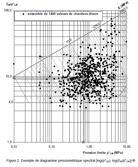
This new form of diagram represents the same points of a large number of diverse, if not disparate, tests in terms of soil types, with the following graphical semiology conventions related to logarithmic scales, compatibility with common paper or screen formats (with the convention of either "portrait" or "landscape"), and the concern to place the range of usual values of soils and weathered rocks at the centre of the graph:

• vertically, 2 logarithmic modules for_EM/ P*LM from 1 to 100
• horizontally, 3 logarithmic moduli for P*LM from 0.01 MPa to 10 MPa;
• At the top, towards the high values of_EM/ P*LM, the straight line [10 / 0.01MPa , 100 / 10MPa] is a "natural" boundary that should not normally be crossed by usual pressuremeter tests;
• At the bottom, towards low values, the physical boundary is_EM/ P*LM = 4 ;
• on the left, towards low P*LM, values below 0.01MPa are difficult to measure and their representation is no longer of interest;
• on the right, the extension of the graph by 1 logarithmic modulus (P*LM up to 100 MPa) or even 2 moduli is possible but the diagram then enters the field of rock mechanics;
• By convention, the graph is in a proportion of 1.15 / 1 (2/√ 3 to 1) ;
• the index lines of the pressuremeter modules are parallel lines in logarithmic spacing, and visually perpendicular to the upper boundary of the graph in the agreed configuration.

The cloud of points representing various tests is indeed centred near the "pivot" value [P*LM =1 MPa ,_EM/ P*LM = 10], and the spread of points around this value is easy to see visually.

Tests with_EM/ P*LM lower than 10 should not be discarded indiscriminately; on the one hand, granular soils without cohesion do give low concavity pressure curves, for which a secant modulus of the order of half the pressure range corresponds to low values for the ratio, on the other hand, for such tests which do not have a pseudo-linear part, the differences in interpretation of the modulus are important, with a tendency to an artificial increase in the modulus in order to conform to an upwardly directed value.

The limit indicated_EM/ P*LM = 4 may seem low, if not lax. It is simply shown that this is the low limit set by definition for a loose granular soil with a maximum void index, whose reaction is linear from p0 to_PLM; such cases exist for clean sand dumped by rainfall, or aggregates slapped under water, for example. Whatever the limit pressure, which is then a function of the mass of soil above the test, the ratio_EM/ P*LM is such that_GM = (Vp+Vp/2) ._PLM/Vp i.e._GM =1.5_PLM and since_EM=8/3GM,_EM = 4_PLM. Finally,_EM/ P*LM is always a little, or even much, lower than_EM/ P*LM.

3. Interest of the spectral pressuremeter diagram ®.

The representation of the results of pressuremeter tests by points in a diagram does not bring new elements compared to those contained in pressuremeter drilling logs, on which the_EM/ P*LM ratio is explicit or implicit. But the gathering of results on the same medium allows a visualization that helps in the synthesis.

3.1 Pedagogical interest

The construction of the diagram was initially done in order to explain to geology students, new to geotechnics, the range of values that the_EM moduli and P*LM pressure limits in soils and rocks could present (Baud, 1991).

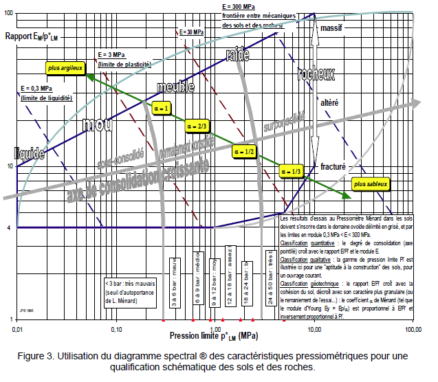
Figure 3 illustrates the presentation in this diagram, extended to the rocky domain (P*LM up to 100MPa), of the notions of classification of soils and rocks, of the clayey or sandy behaviour of the pressiometric response, of the qualification in common language of the compressibility or stiffness of soils (soft, loose, stiff, rocky), and of the assessment by_EM and P*LM of the degree of consolidation.

3.2. Placement of the "regulatory" soil categories in the diagram

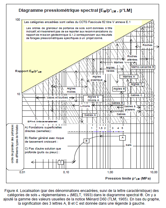
The rules for the use of pressuremeter results for the design of surface and deep foundations (AFNOR 1993; MELT 1993) include the choice for the engineer to classify the values of the measured parameters in very simplified soil categories, defined from the LCPC classification on the one hand, and from the pressuremeter values obtained (essentially_PLM) themselves on the other hand. Although the_EM module is not explicitly used for this categorisation, the examination of the results in the spectral diagram ® can help to make a decision. Figure 4 is an attempt to go further in this categorisation, according to Table 3 of Annex E1 of Fascicule 62, Title V.

With the help of this diagram, it is thus possible to specify the cuts in the "layers" that correspond to groups of homogeneous values in a pile design.

3.3 Site modelling in geotechnical investigation

The use of the Spectral® pressuremeter diagram has proven to be extremely useful for the analysis of complete pressuremeter campaigns, for which the statistical analysis of pressuremeter data and the work on averages is a common method. The grouping or spreading in the diagram of the points characterising formations considered lithologically identical, makes it possible to check their degree of homogeneity, so as to cut out sufficiently homogeneous subsets in the apparent continuum to justify their simplification by representative average values.

Iterations between the borehole logs and the diagram are often necessary to refine the diagnosis. In a well-conducted pressuremeter campaign (or at least with constant "standardised reshuffling"), apparently aberrant or "out-of-cloud" tests may appear and lead to a review of the test reports and lithological sections to check whether these anomalies do not reveal elements of the subsoil structure that did not appear obvious during a rapid analysis of the results.

We suggest the reader to refer to professional journals where we will shortly present in detail some very significant examples.

4. Conclusions and perspectives

The analysis of the results of pressuremeter campaigns using the spectral pressuremeter diagram presented here is only a small addition to the pressuremeter method founded by Louis Ménard, and perfected over the last 50 years by numerous more fundamental theoretical and experimental contributions, such as the lateral friction curves as a function of P*LM (Bustamante and Gianeselli, 1981). It sheds new light on the long-standing problem of determining, or rather evaluating, the rheological coefficient α, for which we hope that it can serve as a support for drawing isovalue curves of this coefficient as a function of_PLM and_EM/P*LM, with the help of both feedback from instrumented foundations and theoretical research.

5. Bibliographic references

AFNOR (1992) Deep foundations for buildings, P11-212 (ex DTU 13.2) Paris laDéfense.

Baud J.-P. (1991) Pressiométrie, "polycopié" de cours de spécialité extérieure, Maîtrise de Sciences et Techniques, Université de Franche-Comté (unpublished).

Bustamante M., Gianeselli L. (1981) Prediction of the bearing capacity of isolated piles under vertical load. Bull. liaison Labo. P. et Ch. ,113, ref. 2536

Lamé G. (1852) Leçons sur la théorie mathématique de l'élasticité des corps solides Bachelier, Paris

Ménard L., Rousseau J. (1962) L'évaluation des compactions, tendances nouvelles. Sols Soils, N°1, Paris

Ministère de l'Equipement, du Logement et des Transports (1993) Règles techniques de conception et de calcul des fondations des ouvrages de génie civil, Cahier des clauses techniques générales applicables aux marchés publics de travaux, Fascicule N°62, Titre V, Textes officiels, imprimerie nationale

Techniques Louis Ménard (1965) Règles d'utilisation des techniques pressiométriques et d'exploitation des résultats obtenus pour le calcul des fondations. Brochure D60 (English translation in Sols Soils N°26, 1975).